• Background
• Approach
• Symbol Definitions
• Core Equations
• Visualization
  • Number of points at various levels of approximation
  • Evaluating via C#
• Daubechies Coefficients
  • Scaling function coefficients
  • Wavelet function coefficients
• Calculation of Scaling Function Initial Values
  • Solving for Initial Values via Python
  • Table of Initial Values
• Calculation of Scaling Function
  • Evaluating the Scaling Function via C#
• Calculation of Wavelet Function
  • Evaluating the Wavelet Function via C#
• Source Code
• References

Background

Daubechies Wavelets are a family of orthogonal wavelets which are recursively-defined. They are discrete functions where each level of approximation fills in midpoints between points across calculated from the previous level and, in the infinite limit, becomes continuous. There are two equivalent nomenclatures: DX and dbX. The db4 (D8) wavelet contains 4 vanishing moments and 8 taps (coefficients) over the non-zero interval $(0,7)$. These are always related by a factor of 2. From here on, only the dbX nomenclature will be used where the wavelet index is X.

Approach

A floating point approach is used for simplicity over the dyadic approach which uses fractional powers of two, $r=n/2^L$, to derive values of r at the next recursion level. A combination of C# and Python were used to generate the figures and data shown. Python was used when necessary for its superior support for matrix solvers. Links to the project’s online source code is provided at the end of the post and is generalized up to at least db10.

This article aims only to demonstrate the calculation of the wavelet and scaling function which are not well-explained in any of the many sources I’ve read. No theory, mathematical proofs, or description of the related wavelet transform will be given as those are covered elsewhere. The db4 wavelet will serve as the primary example here because the db2 wavelet is the dominant example in the literature. Values for wavelets other than db4 will occasionally be given to serve as an aid to general implementation.

Symbol Definitions

𝜑(r) - Scaling function at point r
𝜓(r) - Wavelet function at point r
N - number of Daubechies cofficients for the given wavelet
k - coefficient index
$a_k$ - kth scaling coefficient
$b_k$ - kth wavelet coefficient
$L_x$ - xth level of approximation
$P_x$ - Number of points at the xth level of approximation

Core Equations

Initial Values for Scaling Function
$\{\begin{array}{l}𝜑(r)=\sum _{k=0}^{N-1}{a}_k𝜑(2r-k)\\ \sum \overrightarrow{𝜑}=1\end{array}$

Scaling Function
$𝜑(r)=\sum _{k=0}^{N-1}{a}_k𝜑(2r-k)$

Wavelet Function
$𝜓(r)=\sum _{k=0}^{N-1}{b}_k𝜑(2r-k)$

Visualization

The images below demonstrate db2 and db4 wavelets being recursively filled from 0 to 8 levels of approximation.

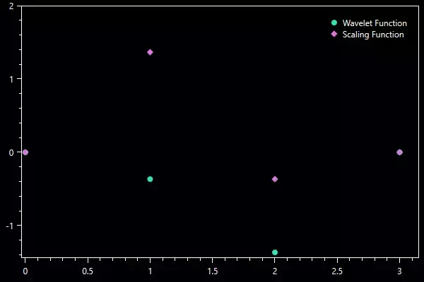
db2 wavelet and scaling functions

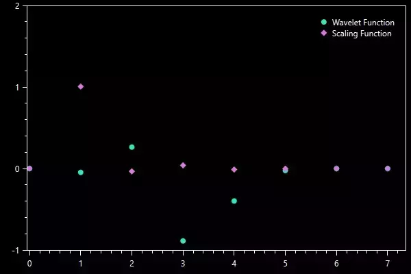
db4 wavelet and scaling functions

Number of points at various levels of approximation

$P_L=P_0\ast 2^L-(2^L-1)$

Evaluating via C#

int PointsAtLevel(int zeroLevelPoints, int level) =>
    zeroLevelPoints * (1 << level) - ((1 << level) - 1);

Daubechies Coefficients

Daubechies coefficients for the scaling function are frequently given in texts and are given here as a table. The calculation of the scaling coefficients may be covered in a future blog. Briefly, the calculation involves a matrix solver with multiple constraints (example) and yields multiple solutions. The final constraint is the convention that the chosen solution is the one which has the largest values front-loaded. This is known as the extremal phase. The sum of coefficients for a given wavelet index is often normalized to 1 and this is the case here.

Scaling function coefficients

Wavelet function coefficients

Wavelet function coefficients are directly derived from the scaling function coefficients via the relationship $b_k=(-1{)}^k\ast a_{N-1-k}$

The db4 wavelet coefficients calculations in detail:

$b_0=(-1{)}^0\ast a_{8-1-0}=1\ast a_7=-0.01498699$
$b_1=(-1{)}^1\ast a_{8-1-1}=-1\ast a_6=-0.0465036$
$b_2=(-1{)}^2\ast a_{8-1-2}=1\ast a_5=0.0436163$
$b_3=(-1{)}^3\ast a_{8-1-3}=-1\ast a_4=0.26450717$
$b_4=(-1{)}^4\ast a_{8-1-4}=1\ast a_3=-0.03957503$
$b_5=(-1{)}^5\ast a_{8-1-5}=-1\ast a_2=-0.89220014$
$b_6=(-1{)}^6\ast a_{8-1-6}=1\ast a_1=1.01094572$
$b_7=(-1{)}^7\ast a_{8-1-7}=-1\ast a_0=-0.32580343$

IEnumerable<float> ToWaveletCoefficients(IEnumerable<float> scalingCoefficients) =>
    scalingCoefficients.Select((coef, index) => index % 2 == 0 ? -coef : coef).Reverse();

Calculation of Scaling Function Initial Values

The scaling function requires values at integer values of r within the wavelet’s range of [0, N-1] with each end of the interval being zero ($𝜑(0)=0,𝜑(N-1)=0$) and all values outside of the interval also being zero. These initial values, $L_0$, are calculated by producing a system of linear equations which can be solved by a constrained matrix solver.

$𝜑(r)=\sum _{k=0}^{N-1}{a}_k𝜑(2r-k)$

And yields the following system of equations for db4:
$𝜑(0)=a_0𝜑(2\ast 0-0)+a_1𝜑(2\ast 0-1)+a_2𝜑(2\ast 0-2)+a_3𝜑(2\ast 0-3)+a_4𝜑(2\ast 0-4)+a_5𝜑(2\ast 0-5)+a_6𝜑(2\ast 0-6)+a_7𝜑(2\ast 0-7)$
$𝜑(1)=a_0𝜑(2\ast 1-0)+a_1𝜑(2\ast 1-1)+a_2𝜑(2\ast 1-2)+a_3𝜑(2\ast 1-3)+a_4𝜑(2\ast 1-4)+a_5𝜑(2\ast 1-5)+a_6𝜑(2\ast 1-6)+a_7𝜑(2\ast 1-7)$
$𝜑(2)=a_0𝜑(2\ast 2-0)+a_1𝜑(2\ast 2-1)+a_2𝜑(2\ast 2-2)+a_3𝜑(2\ast 2-3)+a_4𝜑(2\ast 2-4)+a_5𝜑(2\ast 2-5)+a_6𝜑(2\ast 2-6)+a_7𝜑(2\ast 2-7)$
$𝜑(3)=a_0𝜑(2\ast 3-0)+a_1𝜑(2\ast 3-1)+a_2𝜑(2\ast 3-2)+a_3𝜑(2\ast 3-3)+a_4𝜑(2\ast 3-4)+a_5𝜑(2\ast 3-5)+a_6𝜑(2\ast 3-6)+a_7𝜑(2\ast 3-7)$
$𝜑(4)=a_0𝜑(2\ast 4-0)+a_1𝜑(2\ast 4-1)+a_2𝜑(2\ast 4-2)+a_3𝜑(2\ast 4-3)+a_4𝜑(2\ast 4-4)+a_5𝜑(2\ast 4-5)+a_6𝜑(2\ast 4-6)+a_7𝜑(2\ast 4-7)$
$𝜑(5)=a_0𝜑(2\ast 5-0)+a_1𝜑(2\ast 5-1)+a_2𝜑(2\ast 5-2)+a_3𝜑(2\ast 5-3)+a_4𝜑(2\ast 5-4)+a_5𝜑(2\ast 5-5)+a_6𝜑(2\ast 5-6)+a_7𝜑(2\ast 5-7)$
$𝜑(6)=a_0𝜑(2\ast 6-0)+a_1𝜑(2\ast 6-1)+a_2𝜑(2\ast 6-2)+a_3𝜑(2\ast 6-3)+a_4𝜑(2\ast 6-4)+a_5𝜑(2\ast 6-5)+a_6𝜑(2\ast 6-6)+a_7𝜑(2\ast 6-7)$
$𝜑(7)=a_0𝜑(2\ast 7-0)+a_1𝜑(2\ast 7-1)+a_2𝜑(2\ast 7-2)+a_3𝜑(2\ast 7-3)+a_4𝜑(2\ast 7-4)+a_5𝜑(2\ast 7-5)+a_6𝜑(2\ast 7-6)+a_7𝜑(2\ast 7-7)$

This system can be greatly simplified, given that many values are zero. The endpoints and all other zero values will be removed:
$𝜑(1)=a_0𝜑(2)+a_1𝜑(1)$
$𝜑(2)=a_0𝜑(4)+a_1𝜑(3)+a_2𝜑(2)+a_3𝜑(1)$
$𝜑(3)=a_0𝜑(6)+a_1𝜑(5)+a_2𝜑(4)+a_3𝜑(3)+a_4𝜑(2)+a_5𝜑(1)$
$𝜑(4)=a_2𝜑(6)+a_3𝜑(5)+a_4𝜑(4)+a_5𝜑(3)+a_6𝜑(2)+a_7𝜑(1)$
$𝜑(5)=a_4𝜑(6)+a_5𝜑(5)+a_6𝜑(4)+a_7𝜑(3)$
$𝜑(6)=a_6𝜑(6)+a_7𝜑(5)$

Next, a matrix equation can be written of the form $(\mathbf{A}-\mathbf{I})\overrightarrow{𝜑}=\overrightarrow{0}$ where $\mathbf{I}$ is the identity matrix:

$$\left(\begin{array}{cccccc}{a}_1-1& a_0& 0& 0& 0& 0\\ a_3& a_2-1& a_1& a_0& 0& 0\\ a_5& a_4& a_3-1& a_2& a_1& a_0\\ a_7& a_6& a_5& a_4-1& a_3& a_2\\ 0& 0& a_7& a_6& a_5-1& a_4\\ 0& 0& 0& 0& a_7& a_6-1\end{array}\right)\ast \left(\begin{array}{c}𝜑(1)\\ 𝜑(2)\\ 𝜑(3)\\ 𝜑(4)\\ 𝜑(5)\\ 𝜑(6)\end{array}\right)=\left(\begin{array}{c}0\\ 0\\ 0\\ 0\\ 0\\ 0\end{array}\right)$$

Solving for Initial Values via Python

This matrix equation is solved with the constraint that $\sum \overrightarrow{𝜑}=1$ to find a valid solution. This result also ensures that the integral of the entire scaling function is 1, $\underset{\mathbb{R}}{\int }𝜑=1$. Below, we solve the constrained matrix equation with the scipy.optimize method.

# Helper method for minimization: ||Ax||^2
def f(x):
    y = np.dot(A, x)
    return np.dot(y, y)

# maps 0 or coefficient values to matrix A
def map_index(a, i, j):
    index = 2 * i - j
    if index < 0 or index >= len(a):
        return 0
    else:
        return a[index]

# db4 scaling coefficients
aVector = [ 0.32580343, 1.01094572, 0.89220014, -0.03957503, -0.26450717, 0.0436163, 0.0465036, -0.01498699 ]
N = len(aVector)

A_list = [[map_index(aVector, row, col) for col in range(1, N-1)] for row in range(1, N-1)]
A = np.array(A_list) - np.identity(N - 2)
print(f'A: {A}\n')

zeroVector = np.array(np.zeros(N - 2))

cons = ({'type': 'eq', 'fun': lambda x: x.sum() - 1})
res = optimize.minimize(f, zeroVector, method='SLSQP', constraints=cons, options={'disp' : False})

xbest = res['x']
print(f'db4 initial values: {xbest}\n')
print(f'sum of initial values: {xbest.sum()}')

Table of Initial Values

Calculation of Scaling Function

The scaling function, 𝜑(r), is recursively-defined and requires the initial values from the previous step as well as the Daubechies coefficients. As mentioned in the intro, the function is not continuous until an infinite level of approximations are calculated, so we must settle for a discrete solution.

$$𝜑(r)=\sum _{k=0}^{N-1}{a}_k𝜑(2r-k)$$

The calculation begins by initializing the initial level, $L_0$, by setting all whole integer values to the initial values:

Next, we calculate the values for $L_1$ at the half-integer values:

$𝜑(0.5)=a_0𝜑(1-0)+a_1𝜑(1-1)+a_2𝜑(1-2)+a_3𝜑(1-3)+a_4𝜑(1-4)+a_5𝜑(1-5)+a_6𝜑(1-6)+a_7𝜑(1-7)$
$𝜑(1.5)=a_0𝜑(3-0)+a_1𝜑(3-1)+a_2𝜑(3-2)+a_3𝜑(3-3)+a_4𝜑(3-4)+a_5𝜑(3-5)+a_6𝜑(3-6)+a_7𝜑(3-7)$
$𝜑(2.5)=a_0𝜑(5-0)+a_1𝜑(5-1)+a_2𝜑(5-2)+a_3𝜑(5-3)+a_4𝜑(5-4)+a_5𝜑(5-5)+a_6𝜑(5-6)+a_7𝜑(5-7)$
$𝜑(3.5)=a_0𝜑(7-0)+a_1𝜑(7-1)+a_2𝜑(7-2)+a_3𝜑(7-3)+a_4𝜑(7-4)+a_5𝜑(7-5)+a_6𝜑(7-6)+a_7𝜑(7-7)$
$𝜑(4.5)=a_0𝜑(9-0)+a_1𝜑(9-1)+a_2𝜑(9-2)+a_3𝜑(9-3)+a_4𝜑(9-4)+a_5𝜑(9-5)+a_6𝜑(9-6)+a_7𝜑(9-7)$
$𝜑(5.5)=a_0𝜑(11-0)+a_1𝜑(11-1)+a_2𝜑(11-2)+a_3𝜑(11-3)+a_4𝜑(11-4)+a_5𝜑(11-5)+a_6𝜑(11-6)+a_7𝜑(11-7)$
$𝜑(6.5)=a_0𝜑(13-0)+a_1𝜑(13-1)+a_2𝜑(13-2)+a_3𝜑(13-3)+a_4𝜑(13-4)+a_5𝜑(13-5)+a_6𝜑(13-6)+a_7𝜑(13-7)$

Simplify with the knowledge that for db4, $𝜑(r)=0$ when $r\le 0,r\ge 7$:
$𝜑(0.5)=a_0𝜑(1)=0.3281$
$𝜑(1.5)=a_0𝜑(3)+a_1𝜑(2)+a_2𝜑(1)=0.8773$
$𝜑(2.5)=a_0𝜑(5)+a_1𝜑(4)+a_2𝜑(3)+a_3𝜑(2)+a_4𝜑(1)=-0.2420$
$𝜑(3.5)=a_1𝜑(6)+a_2𝜑(5)+a_3𝜑(4)+a_4𝜑(3)+a_5𝜑(2)+a_6𝜑(1)=0.0343$
$𝜑(4.5)=a_3𝜑(6)+a_4𝜑(5)+a_5𝜑(4)+a_6𝜑(3)+a_7𝜑(2)=0.0022$
$𝜑(5.5)=a_5𝜑(6)+a_6𝜑(5)+a_7𝜑(4)=1.203e-4$
$𝜑(6.5)=a_7𝜑(6)=9.058e-7$

Note that the right-hand side contains known values of 𝜑(r) from the $L_0$ initial values. We will repeat the recursion one additional level to the $L_2$ quarter-integer values:

$𝜑(0.25)=a_0𝜑(0.5-0)+a_1𝜑(0.5-1)+a_2𝜑(0.5-2)+a_3𝜑(0.5-3)+a_4𝜑(0.5-4)+a_5𝜑(0.5-5)+a_6𝜑(0.5-6)+a_7𝜑(0.5-7)$
$𝜑(0.75)=a_0𝜑(1.5-0)+a_1𝜑(1.5-1)+a_2𝜑(1.5-2)+a_3𝜑(1.5-3)+a_4𝜑(1.5-4)+a_5𝜑(1.5-5)+a_6𝜑(1.5-6)+a_7𝜑(1.5-7)$
$𝜑(1.25)=a_0𝜑(2.5-0)+a_1𝜑(2.5-1)+a_2𝜑(2.5-2)+a_3𝜑(2.5-3)+a_4𝜑(2.5-4)+a_5𝜑(2.5-5)+a_6𝜑(2.5-6)+a_7𝜑(2.5-7)$
$𝜑(1.75)=a_0𝜑(3.5-0)+a_1𝜑(3.5-1)+a_2𝜑(3.5-2)+a_3𝜑(3.5-3)+a_4𝜑(3.5-4)+a_5𝜑(3.5-5)+a_6𝜑(3.5-6)+a_7𝜑(3.5-7)$
$𝜑(2.25)=a_0𝜑(4.5-0)+a_1𝜑(4.5-1)+a_2𝜑(4.5-2)+a_3𝜑(4.5-3)+a_4𝜑(4.5-4)+a_5𝜑(4.5-5)+a_6𝜑(4.5-6)+a_7𝜑(4.5-7)$
$𝜑(2.75)=a_0𝜑(5.5-0)+a_1𝜑(5.5-1)+a_2𝜑(5.5-2)+a_3𝜑(5.5-3)+a_4𝜑(5.5-4)+a_5𝜑(5.5-5)+a_6𝜑(5.5-6)+a_7𝜑(5.5-7)$
$𝜑(3.25)=a_0𝜑(6.5-0)+a_1𝜑(6.5-1)+a_2𝜑(6.5-2)+a_3𝜑(6.5-3)+a_4𝜑(6.5-4)+a_5𝜑(6.5-5)+a_6𝜑(6.5-6)+a_7𝜑(6.5-7)$
$𝜑(3.75)=a_0𝜑(7.5-0)+a_1𝜑(7.5-1)+a_2𝜑(7.5-2)+a_3𝜑(7.5-3)+a_4𝜑(7.5-4)+a_5𝜑(7.5-5)+a_6𝜑(7.5-6)+a_7𝜑(7.5-7)$
$𝜑(4.25)=a_0𝜑(8.5-0)+a_1𝜑(8.5-1)+a_2𝜑(8.5-2)+a_3𝜑(8.5-3)+a_4𝜑(8.5-4)+a_5𝜑(8.5-5)+a_6𝜑(8.5-6)+a_7𝜑(8.5-7)$
$𝜑(4.75)=a_0𝜑(9.5-0)+a_1𝜑(9.5-1)+a_2𝜑(9.5-2)+a_3𝜑(9.5-3)+a_4𝜑(9.5-4)+a_5𝜑(9.5-5)+a_6𝜑(9.5-6)+a_7𝜑(9.5-7)$
$𝜑(5.25)=a_0𝜑(10.5-0)+a_1𝜑(10.5-1)+a_2𝜑(10.5-2)+a_3𝜑(10.5-3)+a_4𝜑(10.5-4)+a_5𝜑(10.5-5)+a_6𝜑(10.5-6)+a_7𝜑(10.5-7)$
$𝜑(5.75)=a_0𝜑(11.5-0)+a_1𝜑(11.5-1)+a_2𝜑(11.5-2)+a_3𝜑(11.5-3)+a_4𝜑(11.5-4)+a_5𝜑(11.5-5)+a_6𝜑(11.5-6)+a_7𝜑(11.5-7)$
$𝜑(6.25)=a_0𝜑(12.5-0)+a_1𝜑(12.5-1)+a_2𝜑(12.5-2)+a_3𝜑(12.5-3)+a_4𝜑(12.5-4)+a_5𝜑(12.5-5)+a_6𝜑(12.5-6)+a_7𝜑(12.5-7)$
$𝜑(6.75)=a_0𝜑(13.5-0)+a_1𝜑(13.5-1)+a_2𝜑(13.5-2)+a_3𝜑(13.5-3)+a_4𝜑(13.5-4)+a_5𝜑(13.5-5)+a_6𝜑(13.5-6)+a_7𝜑(13.5-7)$

Then simplify:

$𝜑(0.25)=a_0𝜑(0.5)$
$𝜑(0.75)=a_0𝜑(1.5)+a_1𝜑(0.5)$
$𝜑(1.25)=a_0𝜑(2.5)+a_1𝜑(1.5)+a_2𝜑(0.5)$
$𝜑(1.75)=a_0𝜑(3.5)+a_1𝜑(2.5)+a_2𝜑(1.5)+a_3𝜑(0.5)$
$𝜑(2.25)=a_0𝜑(4.5)+a_1𝜑(3.5)+a_2𝜑(2.5)+a_3𝜑(1.5)+a_4𝜑(0.5)$
$𝜑(2.75)=a_0𝜑(5.5)+a_1𝜑(4.5)+a_2𝜑(3.5)+a_3𝜑(2.5)+a_4𝜑(1.5)+a_5𝜑(0.5)$
$𝜑(3.25)=a_0𝜑(6.5)+a_1𝜑(5.5)+a_2𝜑(4.5)+a_3𝜑(3.5)+a_4𝜑(2.5)+a_5𝜑(1.5)+a_6𝜑(0.5)$
$𝜑(3.75)=a_1𝜑(6.5)+a_2𝜑(5.5)+a_3𝜑(4.5)+a_4𝜑(3.5)+a_5𝜑(2.5)+a_6𝜑(1.5)+a_7𝜑(0.5)$
$𝜑(4.25)=a_2𝜑(6.5)+a_3𝜑(5.5)+a_4𝜑(4.5)+a_5𝜑(3.5)+a_6𝜑(2.5)+a_7𝜑(1.5)$
$𝜑(4.75)=a_3𝜑(6.5)+a_4𝜑(5.5)+a_5𝜑(4.5)+a_6𝜑(3.5)+a_7𝜑(2.5)$
$𝜑(5.25)=a_4𝜑(6.5)+a_5𝜑(5.5)+a_6𝜑(4.5)+a_7𝜑(3.5)$
$𝜑(5.75)=a_5𝜑(6.5)+a_6𝜑(5.5)+a_7𝜑(4.5)$
$𝜑(6.25)=a_6𝜑(6.5)+a_7𝜑(5.5)$
$𝜑(6.75)=a_7𝜑(6.5)$

Once again, all of the values of 𝜑(r) required to evaluate the right-hand side were calculated during the previous step. The solutions for $L_0$ to $L_2$ are compiled in the following tables:

Evaluating the Scaling Function via C#

An iterative approach is used here rather than a true recursive method. The following method calculates the scaling function’s next level of approximation and is valid for $L>0$. $L_0$ must be separately calculated as described by the Initial Values section.

Vector2[] GetScalingLevel(int level, Vector2[] previous, float[] scalingCoefs)
{
    var scaling = new Vector2[PointsAtLevel(scalingCoefs.Length, level)];
    float maxRange = scalingCoefs.Length - 1f;
    float distancePerIndex = maxRange / (scaling.Length - 1);

    for (int n = 0; n < scaling.Length; n += 2)
        scaling[n] = previous[n / 2];

    for (int n = 1; n < scaling.Length; n += 2)
    {
        float sum = 0;
        float r = n / (float)(1 << level);

        for (int k = 0; k < scalingCoefs.Length; k++)
        {
            float rPrevious = 2 * r - k;
            int rIndex = (int)MathF.Round(rPrevious / distancePerIndex);

            if (rPrevious >= 0 && rPrevious <= maxRange)
                sum += scalingCoefs[k] * scaling[rIndex].Y;
        }
        scaling[n] = new Vector2(r, sum);
    }

    return scaling;
}

Calculation of Wavelet Function

The wavelet function, 𝜓(r), is more straightforward once the scaling function has been calculated. Its equation is given by:

$$𝜓(r)=\sum _{k=0}^{N-1}{b}_k𝜑(2r-k)$$

Given that $L_2$ was previously calculated for the scaling function, the same values of r can be evaluated for the wavelet function at $L_2$:

$𝜓(0.25)=b_0𝜑(0.5-0)+b_1𝜑(0.5-1)+b_2𝜑(0.5-2)+b_3𝜑(0.5-3)+b_4𝜑(0.5-4)+b_5𝜑(0.5-5)+b_6𝜑(0.5-6)+b_7𝜑(0.5-7)$
$𝜓(0.5)=b_0𝜑(1-0)+b_1𝜑(1-1)+b_2𝜑(1-2)+b_3𝜑(1-3)+b_4𝜑(1-4)+b_5𝜑(1-5)+b_6𝜑(1-6)+b_7𝜑(1-7)$
$𝜓(0.75)=b_0𝜑(1.5-0)+b_1𝜑(1.5-1)+b_2𝜑(1.5-2)+b_3𝜑(1.5-3)+b_4𝜑(1.5-4)+b_5𝜑(1.5-5)+b_6𝜑(1.5-6)+b_7𝜑(1.5-7)$
$𝜓(1)=b_0𝜑(2-0)+b_1𝜑(2-1)+b_2𝜑(2-2)+b_3𝜑(2-3)+b_4𝜑(2-4)+b_5𝜑(2-5)+b_6𝜑(2-6)+b_7𝜑(2-7)$
…
$𝜓(6.5)=b_0𝜑(13-0)+b_1𝜑(13-1)+b_2𝜑(13-2)+b_3𝜑(13-3)+b_4𝜑(13-4)+b_5𝜑(13-5)+b_6𝜑(13-6)+b_7𝜑(13-7)$
$𝜓(6.75)=b_0𝜑(13.5-0)+b_1𝜑(13.5-1)+b_2𝜑(13.5-2)+b_3𝜑(13.5-3)+b_4𝜑(13.5-4)+b_5𝜑(13.5-5)+b_6𝜑(13.5-6)+b_7𝜑(13.5-7)$

And simplifies to:

$𝜓(0.25)=b_0𝜑(0.5)$
$𝜓(0.5)=b_0𝜑(1)$
$𝜓(0.75)=b_0𝜑(1.5)+b_1𝜑(0.5)$
$𝜓(1)=b_0𝜑(2)+b_1𝜑(1)$
…
$𝜓(6.5)=b_7𝜑(6)$
$𝜓(6.75)=b_7𝜑(6.5)$

Evaluating the Wavelet Function via C#

The wavelet function code is very similar to the scaling function code. The level is baked into scaling and isn’t required.

Vector2[] GetWaveletLevel(Vector2[] scaling, float[] waveletCoefs)
{
    var wavelet = new Vector2[scaling.Length];

    float maxRange = waveletCoefs.Length - 1f;
    float distancePerPoint = maxRange / (wavelet.Length - 1);

    for (int n = 0; n < wavelet.Length; n++)
    {
        float sum = 0;
        float r = n * distancePerPoint;

        for (int k = 0; k < waveletCoefs.Length; k++)
        {
            float rPrevious = 2 * r - k;
            int rIndex = (int)MathF.Round(rPrevious / distancePerPoint);

            if (rPrevious >= 0 && rPrevious <= maxRange)
                sum += waveletCoefs[k] * scaling[rIndex].Y;
        }
        wavelet[n] = new Vector2(r, sum);
    }

    return wavelet;
}

Source Code

Main Project
Scaling and Wavelet Function (C#))
Initial Scaling Values (Python)

References

Wavelets Made Easy - Yves Nievergelt (2001)
Wavelet Browser - PyWavelets